I studied stochastic processes as part of my master’s degree, but that was a while ago and I’ve forgotten a lot, so when I saw a Stastical Mechanics course appear on Coursera I couldn’t resist. The first week covers some methods (albeit inefficient) for calculating 𝛑.

Direct sampling Monte Carlo

1
2
3
4
5
6
7
8
9
10
11

function mc_pi(N)
    n_hits = 0
    for i = 1:N
        x = rand() * 2 - 1
        y = rand() * 2 - 1
        if x^2 + y^2 < 1
            n_hits += 1
        end
    end
    4 * n_hits / N
end

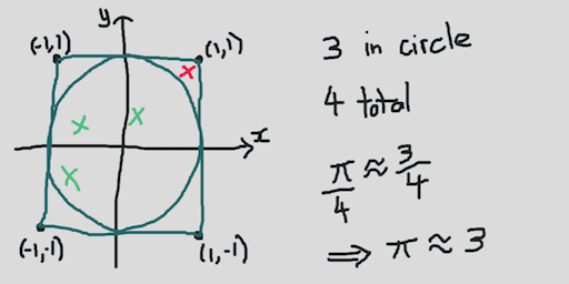
This picks an (x, y) coordinate in the rectangle bounded by x=-1, x=1, y=-1, y=1 N times. Each time, we check if the point lands in the unit circle. The ratio of the areas of the circle and square is 𝛑/4, so we can use 4 * n_hits / N to approximate 𝛑.

Markov chain Monte Carlo

This example doesn’t highlight the weaknesses of direct sampling, but if we are dealing with non-rectangular regions or higher dimensional spaces, it is less practical to implement. In these cases a random walk walk may work better (although I’ll stick to a 2D squares for simplicity in my examples).

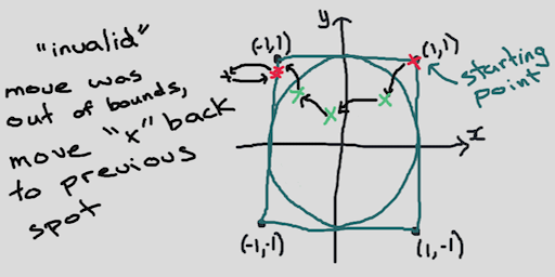
Rather than sampling points directly, we pick a sequence of points via a random walk; these either fall inside or outside of the unit circle and can then be used to approximate 𝛑. However, there is a possibility that the random walk may take us outside the sampling region, and the algorithm has to deal with it appropriately.

Here is the algorithm demonstrated in the Coursera class, translated into Julia. I was pretty surprised when I saw it…

1
2
3
4
5
6
7
8
9
10
11
12
13
14
15

function markov_pi(N, delta)
    x, y = 1.0, 1.0
    n_hits = 0
    for i = 1:N
        del_x = (rand() - 0.5) * 0.5 * delta
        del_y = (rand() - 0.5) * 0.5 * delta
        if (abs(x + del_x) < 1.0) && (abs(y + del_y) < 1.0)
            x, y = x + del_x, y + del_y
        end
        if x^2 + y^2 < 1
            n_hits += 1
        end
    end
    4 * n_hits / N
end

When the walk lands at a point that is “out of bounds”, it simply pretends that our marker hasn’t moved, but it still counts that as one iteration of the sequence. So that point is counted twice, or even more if it goes out of bounds again! (Gasp)

This really confused me for a few minutes, but I had a flash of intuition – helped by the lectures, of course :)

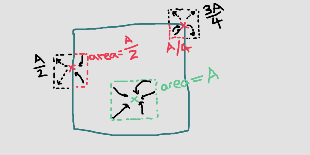
When we land near an edge position there is a chance we will stay there, but this is conditional upon us landing there in the first place. Conveniently, the chance that we move out of bounds and remain at the same spot precisely counteracts the reduced probability of landing near the edges.

The green point in the center has a “catchment area” of A, but upon landing, we move to a new spot with probability 1. The point on the left side has half the catchment area, however, if we land there we expect to stay for one extra move (½ + ¼ + 1/8 + …). Similarly, the point in the top right has ¼ the catchment area, but if we land there we expect to remain for an extra 3 moves (¾ + 9/16 + 27/64 + …).

As mentioned in the title, this was a pretty handwavey explanation, but I was impressed that such a simple algorithm corrects its own “flaws”. A more detailed explanation can be found in Wikipedia.